Rocket Lab

Purpose

To determine the trajectory of a model rocket.

Equipment

PASCO Rocket Engine Test Bracket, dual range force probe, iron ring stand, Estes B6 or C6 motor, Logger Pro

Procedure

After setting up the model rocket engine on a stable platform, open logger pro. 
     Select EXPERIMENT, then DATA COLLECTION. 
     Set duration to 3 seconds. 
     Set sampling rate to 1000 samples/second.

Click the TRIGGERING tab. 
     Select triggering. 
     Select decreasing. 
     Set trigger force to -0.2 Newtons

BE SURE TO CLEAR THE AREA AROUND THE EXPERIMENTAL SET UP!
     Set the zero force probe.
     Click the collect data icon (you should observe "waiting for trigger and data..." within the top portion of the graph area)
     Once the area is clear, ignite the motor

After the motor has stopped. You should be able to see a graph of force vs time. From the graph, make your assumptions on a few questions.

The questions are as follows:

1. Draw a system schema and force diagram and apply Newton's Second Law to a rocket on the launch pad.

2. Redraw the system schema and force diagram and a statement of Newton's Second Law based on this force diagram for the moment the rocket leaves the ground.

     a. What agent is causing the upward force?

     b. Do you think the thrust force is constant? Explain.

3. As the fuel burns, is your rocket speeding up or slowing down? Which force has to be bigger for this to occur? Do you need to modify your force diagram?

4. Your rocket is not a particle. Do you think you have to deal with air resistance? Redo your system schema, force diagram, and statement of Newton's Second Law to include it.

5. Do you think F(air) is constant? If not. what does it depend on?

6. When the rocket has run out of fuel, what direction is still going? Is it speeding up or slowing down? Based on this, what does your force diagram look like now? What is your new statement of Newton's Second Law?

7. How will you know when the rocket reaches its highest point?

8. Get your answers on your boards.

We will use the ideas the class has developed to make a model to figure out how high a real rocket actually goes. We will test your model against experimental data.

9. What specific information and measurements do we need? Be sure to distinguish what quantities need to be looked up and what needs to be measured to do the calculations for your model.

10. Now you will need to obtain the thrust vs time data for a rocket motor. Ultimately, this data will be used to help calculate the height of the rocket flight. Not all of the data that you obtain will be useful for the calculations in your model. Think carefully about which data to include. Consider this: Does the rocket accelerate instantaneously or does the thrust take time to build?

Once you have answered all the questions and collected your experimental data, it is time to launch a real rocket. For this lab, the measurements needed for the maximum height include: mass = 0.0632 kg, diameter = 0.02441 m, delta t = 0.001 s, F(g) = 0.6194, rho = 1.2.

Create an excel spreadsheet with the columns: time (s), F(thrust)(N), a (m/s/s), v (m/s), rhoAv^2 (N), delta r (m), r (m). Set up the spreadsheet with these formulas: a = ( F(thrust) - F(g) - rhoAv^2) / mass , v(final) = v(initial) + a(delta t) , delta r = (v(final)^2 - v(initial)^2) / 2a

Once you have the spreadsheet set up, go to your experimental data table and select the times in which the thrust force is greater than the force of gravity of the rocket (which is 0.6194 N). Select as much time as needed along with the corresponding thrust values. Include the values where thrust is less than gravity at this point. Put those values in the excel spreadsheet. Add the desired constants and make the excel formula based on the written formulas above. Be sure to add the $ symbol before the letter and number of the cell with a constant value. Your table should look like this:

At first, the height values are very small, but this is fine because this happens in the first few seconds of flight. Once more time and thrust values are added, there is a significant change in height. This is where the maximum height can be found. The next two pictures show the maximum height.

The maximum height for this lab is approximately 147.26 m.

Human Power

Purpose

To determine the power output of a person.

Equipment

Two meter sticks, stopwatch, force plate or kilogram bathroom scale.

Introduction

Power is defined to be the rate at which work is done or equivalently, the rate at which energy is converted from one form to another. In this experiment, you will do some work by climbing from the first floor of the science building to the second floor. By measuring the vertical height climbed and knowing your mass, the change in your gravitational potential energy can be found:

Δ PE = mgΔh

Where m is the mass in kg, g is the acceleration of gravity in m/s/s, and h is the vertical height gained. Your output power can be determined by:

Power = Δ PE / Δt

Where Δt is the time it takes to climb the vertical height h.

Procedure

1. Determine your mass by weighing on the kilogram bathroom scale or force plate. Record your mass in kg or your force due to gravity in N.

- Since Potential Energy requires mass, acceleration due to gravity, and a vertical height, mass and gravity can be combined to get the force of gravity on the person by using the formula F_g = mg.

2. Measure the vertical distance between the ground floor and the second floor for the science building. This can most easily be done by using two meter sticks held end to end in the stairwell.

-This was done using the two meter sticks end to end and stacking them from the floor of the ground floor to the floor of the second floor.

3. Designate a record keeper and a timer for the class. At the command of the timing person, run or walk (whatever you feel comfortable doing) up the stairs from the ground floor to the second floor. Be sure that your name and time are recorded by the record keeper.

4. After everyone in the class has completed one trip up the stairs, repeat for one more trial.

5. Return to class and calculate your personal power output in watts using the data collected from each of your climbing trips up the stairs. Obtain the average power output from the two trials.

-F_g = 770 N        -T₁ = 5.82 s      -Δt = 6.01 s

-Δh = 4.26 m      -T₂ = 6.19 s      -1 hp = 746 watts

Power = (mg)Δh/Δt = (770 N)(4.26 m)/(6.01 s) = 545.79 watts

6. Put your average power on the board and then calculate the average power for the entire class once everyone has reported their numbers on the board.

-Average power of class = 0.7 hp

7. Determine your average power output in units of horsepower.

-545.79 watts = 0.7316 hp

Questions

1. Is it okay to use your hands and arms on the railing to assist you in your climb up the stairs? Explain why or why not.

-It is okay to use your hands and arms to assist in climbing the stairs because it shortens the time taken to climb the stairs. Since mass, gravity, and height don't change when calculating the power, time is all that's left that could change the power output. When time is shortened, power is increased. When you use the handrail to aid you in climbing, you are exerting additional power to climb, and therefore shorten the time. Walking up will take longer thereby decreasing the power output. 

2. Discuss some of the problems with the accuracy of this experiment.

-Some problems in the accuracy of the experiment may include: inconsistent climbing style for the class (running vs. walking, stepping on individual steps vs. skipping steps), human error in measurement (height, time)

Drag Force on A Coffee Filter

Purpose

To study the relationship between air drag forces and the velocity of a falling body.

Equipment

Computer with Logger Pro software, Lab Pro, motion detector, nine (9) coffee filters, meter stick

Introduction

When an object moves through a fluid, such as air, it experiences a drag force that opposes its motion. This force generally increases with the velocity of the object. In this lab, we are going to investigate the velocity dependence of the drag force. We will start by assuming the drag force, F_D has a simple power law dependence on the speed given by the formula:

F_D = k |V|ⁿ, where the power n is to be determined by the experiment.

This lab will investigate drag forces acting on a falling coffee filter. Because of the large surface area and low mass of these filters, they reach terminal speed soon after being released.

Procedure

You will be given a packet of nine (9) nested coffee filters. It is important that the shape of this packet stays the same throughout the experiment so do not take the filters apart or otherwise alter the shape of the packet. Why is it important for the shape to stay the same? Explain and use a diagram.

-The reason why the shape of the packet has to stay the same throughout the experiment is to have consistent data. If the packet has a different shape, the drag force on the packet would be different.

-This picture shows that if the packet was flattened, there would be more air resistance and drag force. To keep the results consistent, the packet's shape should not be altered.

1. Login to your computer with username. Start the Logger Pro software, open the Mechanics folder and the graphlab file. Don't forget to label the axes of the graph and create an appropriate title for the graph. Set the data collection rate to 30 Hz.

2. Place the motion detector on the floor facing upward and hold the packet of nine (9) filters at a minimum height of 1.5 meters directly above the motion detector. (Be aware of any nearby objects which can cause reflections.) Start the computer collecting data, and then release the packet. What should the Position vs Time graph look like? Explain.

-This is my prediction on what Position vs Time should look like. The origin would be the motion detector. Since the packet is falling, the motion would be going to the 0 meter mark in less than a second.

Verify that the data are consistent. If not, repeat the trial. Examine the graph and using the mouse, select (click and drag) a small range of data points near the end of the motion where the packet moved with constant speed. Exclude and early or late points where the motion is not uniform.

3. Use the curve fitting option from the analysis menu to fit a linear curve (y = mx + b) to the selected data. Record the slope (m) of the curve from this fit. What should this slope represent? Explain.

-This is a graph of one of the trials we did. The slope represents the velocity. My earlier prediction was wrong because the velocity is fairly constant the instant the packet was released; it did not curve unlike in my prediction.

Repeat this measurement at least four more times, and calculate the average velocity. Record all data in an excel table.

4. Carefully remove one filter from the packet and repeat the procedure in parts 2 and 3 for the remaining packet of eight (8) filters. Keep removing filters one at a time and repeating the above steps until you finish with a single coffee filter. Print a copy of one of your best x vs t graphs that show the motion and the linear curve fit data for everyone in your group (Do not include the data table; graph only please).

-This is the data sheet of all the trials we did from nine (9) filters to one (1) filter. All these values are the velocities in m/s. We used the average velocity as the terminal velocity for that set of filters.

5. In Graphical Analysis, create a two column data table with packet weight (number of filters) in one column and the average terminal speed (|V|) in the other. Make a plot of packet weight (y-axis) vs. terminal speed not velocity (x-axis). Choose appropriate labels and scales for the axes of your graph. Be sure to remove the "connecting lines" from the plot. Perform a Power Law fit of the data and record the power, n, given by the computer. Obtain a printout of your graph for each member of your group. (Check the % error between your experimentally determined n and the theoretical value before you make a printout - you may need to repeat trials if the error is too large.)

-This is our power law fit of the experiment. The number of filters is the y-axis and the average terminal speed is the x-axis. Our n is 2.68, which is considerably larger than the theoretical value of 2. Our percent error was 34% . I believe this happened due to human error. One of my groupmates in charge of data collection may have included data points outside of the sloped lines in the position vs time graphs, thereby increasing the terminal velocities.

6. Since the drag force is equal to the packet weight, we have found the dependence of drag force on speed. Write equation 1 above with the value of n obtained from your experiment. Put a box around this equation. Look in the section of drag forces in your text and write down the equation given there for the drag force on an object moving through a fluid. How does your value of n compare with the value given in the text? What does the other fit parameter represent? Explain.

-This lab's formula for drag force: F_D = k |V|ⁿ
-Another formula for drag force: F_D = (1/2) ρ υ² C_D A, where F_D is the drag force, ρ is the mass density of the fluid, υ is the velocity of the object relative to the fluid, A is the reference area, and C_D is the drag coefficient.
-Our value for n is significantly different from the one in the text.
-The other parameter, k, is the mass of the packet.

Conclusion

In this lab experiment, I've learned how to calculate drag force using the formula: F_D = k |V|ⁿ. I've also learned how to find the terminal speeds of objects and use the computer to determine the value of n.

Sources of error include: improper data measurement by using data from the edges of the sloped lines in the position vs time graphs, inconsistent handling of packet which includes varying drop heights and packet landing to the side of the motion detector, and lack of additional trials to gather the best data.

*Author's Notes*
-Hand-drawn figures aren't drawn to scale.

Working with Spreadsheets

 Purpose:

The purpose of this laboratory exercise is to get familiar with electronic spreadsheets by using them in some simple applications.

Equipment:

Computer with Microsoft Excel software.

Procedure:

1. Your instructor will give you a brief explanation of how a spreadsheet works and show you some of the basic operations and functions.

2. Open the Microsoft Excel program.

3. Create a simple spreadsheet that calculates the following function: f(x) = A sin(Bx + C). Your experimental values are A = 5, B = 3, and C = π/3. Place these values at the right side of the spreadsheet in the region reserved for constants. Put the words amplitude, frequency, and phase next to each as an explanation for the meaning of each constant. Place column headings for "x" and "f(x)" near the middle of the spreadsheet, enter a zero in the cell below "x", and enter the formula shown above in the cell below "f(x)". Be sure to put an equal sign in front of the formula. Create a column for values of x that run from zero to 10 radians in steps of 0.1 radians. Use the copy feature to create these x values. Similarly, create in the next column the corresponding values of f(x) by copying the formula shown above down through the same number of rows.

*Author's note: Use the dollar ($) sign before the letter and number designation of the cell that you want the value to remain constant. This is because the copy feature will include the empty cells beneath your constant values (e.g. A = 5, B = 3, C = π/3). The resulting values under the "f(x)" column will not be the values you need.

4. Once the generated data looks reasonable, copy this data onto a clipboard by highlighting the contents of the two columns and choosing EDIT => COPY from the menu bar. Print out a copy of your spreadsheet (the first 20 rows or so) and also print out the spreadsheet formulas (press CTRL ~).

*Note that in the "x" column, the formulas are: =[previous cell] + 0.1. The formulas in the "f(x) column are: =$E$3*SIN($F$3*[corresponding "x" column cell]+$G$3). The dollar signs ($) before the letter and number designation of the cells E3, F3, and G3 mean that the values of cells E3, F3, and G3 are constant throughout the copying process. The only value that changes is that of the cells in the "x" column.

5. Minimize the spreadsheet window and run the Graphical Analysis program by opening the Physics Apps icon and double-click the Graphical Analysis icon. Once the program loads, click on the top of the "x" column then choose EDIT => PASTE to place the data from the clipboard into your graphing program. A graph of the data should appear in the graph window. Put appropriate labels on the horizontal and vertical axes of the graph.

6. Highlight the portion of the graph you want to analyze and choose ANALYZE => CURVE FIT from the menu bar to direct the computer to find a function that best fits the data. From the list of possible functions, give the computer a hint as to what type of function you expect your data to match. The computer should display a value for A, B, and C that fit the sine curve that you are plotting. Make a copy of the data and graph by selecting FILE => PRINT.

7. Repeat the above process for a spreadsheet that calculates the position of a freely falling particle as a function of time. This time, your constants should include the acceleration of gravity (g = 9.8 m/s²), the initial position (x₀ = 1000 m), initial velocity (v₀ = 50 m/s), and the time increment (Δt = 0.2 s). Print out the spreadsheet (Resulting values and formulas). Again, copy the data into the Graphical Analysis program and obtain a graph of position vs time. Fit this data to a function (y = A + Bx + Cx²) which closely matches the data. Get the print out of this graph with the data table.

Conclusion:

In this lab exercise, I've learned how to properly write certain formulas into Excel. I did not know the functionality of the dollar sign ($) before this exercise. I've also learned how to properly calculate and transfer data from Excel to the Graphical Analysis program. This exercise is not limited to linear or quadratic formulas. You can create a complex formula and Excel will calculate the data with the given parameters and limitations.

Acceleration Lab

Fig. 1: Acceleration of Gravity page 1

Fig. 2: Acceleration of Gravity page 2

  

Today's lab experiment was about acceleration due to gravity. Our materials were a ball, a wire basket, a motion detector, Lab Pro interface, Logger Pro software, and a windows-based computer.

The goal of this lab was to use the computer to collect position vs time data for a rubber ball tossed into the air. The position vs time graph can be changed to a velocity vs time graph of the motion of the ball.

We connected the motion detector to the lab pro to the computer and booted up the Logger Pro software. We opened the graphlab file and the position vs time graph was set. Before tossing the ball, we clicked the COLLECT button to make sure that the motion of the bal does not go unrecorded. The motion detector works by sending sound waves parallel to the emitting face. As the sound waves travel through the air, any object going above the motion detector will reflect the sound waves back to it. The Logger Pro software then reads the data from the detector and plots it in a graph.

The data we needed depended on how well did we toss the ball over the motion detector. We did many, MANY trial tests to get the right graphs.

Fig. 3: Position vs Time Graph

   

The above picture is one of three graphs we took our data from. This is the Position vs Time graph. The highlighted region is part of a parabola from which we got our data for the column labelled "gexp2a" on our table. The irregular motion of the ball and the hands of one of my groupmates before releasing the ball above the detector is represented by the data before the highlighted region. The data after the highlighted region is the motion of the ball hitting the wire grate above the motion detector.

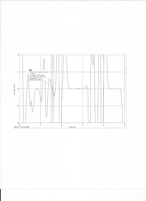
Fig. 4: Velocity vs Time graph

This picture is one of three Velocity vs Time graphs derived from the Position vs Time graphs. This graph is the derivative of the P vs T graph above it. We put the data we gathered from the V vs T graphs in the column labeled "gexp(m)".

All of the data we collected is in Figure 2 in the table titled "Results from Falling Body Experiment".

In conclusion, we graphed the motion of a ball free-falling over a motion detector. The position graph shows the distance between the ball and the motion detector. The derivative of the position graph is the velocity graph. When a parabola is plotted in a position graph, a sloped line is plotted in its derived velocity graph. There were many sources of error such as varying distance between the ball and the motion detector, improper release of the ball, poor grate and detector placement, and inconsistent ball motion and direction above the detector.