 |
| Fig. 1: Acceleration of Gravity page 1 |
 |
| Fig. 2: Acceleration of Gravity page 2 |
Today's lab experiment was about acceleration due to gravity. Our materials were a ball, a wire basket, a motion detector, Lab Pro interface, Logger Pro software, and a windows-based computer.
The goal of this lab was to use the computer to collect position vs time data for a rubber ball tossed into the air. The position vs time graph can be changed to a velocity vs time graph of the motion of the ball.
We connected the motion detector to the lab pro to the computer and booted up the Logger Pro software. We opened the graphlab file and the position vs time graph was set. Before tossing the ball, we clicked the COLLECT button to make sure that the motion of the bal does not go unrecorded. The motion detector works by sending sound waves parallel to the emitting face. As the sound waves travel through the air, any object going above the motion detector will reflect the sound waves back to it. The Logger Pro software then reads the data from the detector and plots it in a graph.
The data we needed depended on how well did we toss the ball over the motion detector. We did many, MANY trial tests to get the right graphs.
 |
| Fig. 3: Position vs Time Graph |
The above picture is one of three graphs we took our data from. This is the Position vs Time graph. The highlighted region is part of a parabola from which we got our data for the column labelled "gexp2a" on our table. The irregular motion of the ball and the hands of one of my groupmates before releasing the ball above the detector is represented by the data before the highlighted region. The data after the highlighted region is the motion of the ball hitting the wire grate above the motion detector.
 |
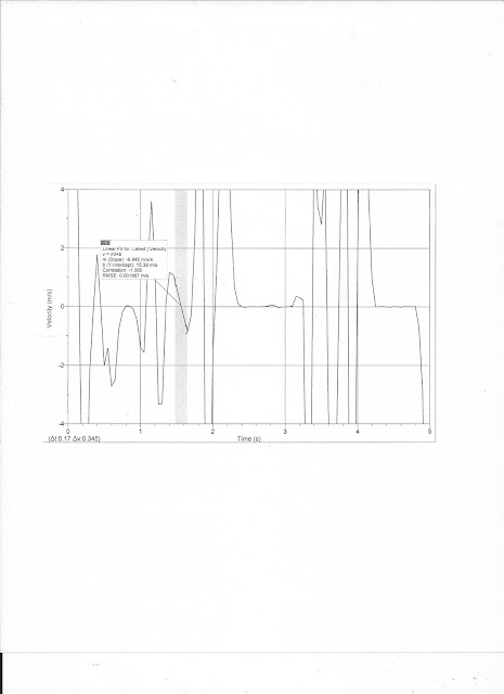
| Fig. 4: Velocity vs Time graph |
This picture is one of three Velocity vs Time graphs derived from the Position vs Time graphs. This graph is the derivative of the P vs T graph above it. We put the data we gathered from the V vs T graphs in the column labeled "gexp(m)".
All of the data we collected is in Figure 2 in the table titled "Results from Falling Body Experiment".
In conclusion, we graphed the motion of a ball free-falling over a motion detector. The position graph shows the distance between the ball and the motion detector. The derivative of the position graph is the velocity graph. When a parabola is plotted in a position graph, a sloped line is plotted in its derived velocity graph. There were many sources of error such as varying distance between the ball and the motion detector, improper release of the ball, poor grate and detector placement, and inconsistent ball motion and direction above the detector.